Hierarcical clustering

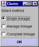
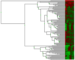
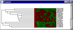
Hierarcical clustering was the first analysis method implemented in this program. That is why the result will apear in the main window. The theory behind this type of clustering is simply to group similar data and represent the group as it's members closest vector (Single linkage), the average of all members' vectors (average linkage) or the vector furthest from the reference point (complete linkage). Usually litterature describes two such methods of grouping data, eighter agglomerative or divisive. The latter starts by defining the complete set as a group and dividing it until each vector has a group of its own.An agglomerative approach starts in the other end and terminates when all vectors are member og the same group. The method implemented here are agglomerative. The hierarcical clustering method is very computation intensive and demands a lot of computer memory due to it's computation of a distance-matrix. This matrix is required for storing the distance (euclidean) from each vector to all the others, hence a dataset containg 6000 genes will result in a triangular 6000*6000 distance matrix that has to be traversed for each gene in the building of a hieracical tree. There has been made a great effort in finding ways to minimize computation time and memory in the algorithm used by this program. (The runtime and memory requirement is actually a fraction of what it was when the first version was tested). Further descriptions of the hierarcical method of clustering data will not be discussed here. The "Select method" dialog will appeare once the clustering button is clicked. From this it is possible to select one of the methods described above. After the requested clustering method has been selected, the program will start calculating a distance matrix, building a cluster tree (dendrogram) and preparing the result in an image. This usually takes a while, especialy if the dataset is large. The statusbar will tell where in the process the program is at all time. The dendrogram The dendrogram is displayed as a tree which ends up in a color code of the actual data. This colorcode is a small square for each element in the vector representing the gene. A red square represent a positive value, and negative values are colored green. The intensity of the color is a measure of the relative difference between other values at the same side of zero. For example, the lowest values will have the lightest green color, and the highest ones the lightest red. A cluster will always have two directly connected components, eighter two other clusters or two vectors (leaf nodes) or one of each. The length of the horisontal lines that connect two clusters (nodes) are a measure of how relatively close they are (calculated with euclidean distances). Each cluster that contains two other clusters has a green square in the middle. By clicking this square, it is possible to zoom in on this sub-cluster. If the selected set does not contain over a certain number of vectors (genes) a zoomwindow will appear. The zoomwindow is the same dendrogram as described above, only the squares are larger, and the names of each gene will be written to the right of the colorcode. Both the complete clusterimage in the main window and the zoomed image can be saved to a gif-file by selecting save-clusterimage or save-zoomimage from the file menu. It should be possible to find shared expression patterns just by looking at the color codes of closely clustered elements.