Self-Organizing map

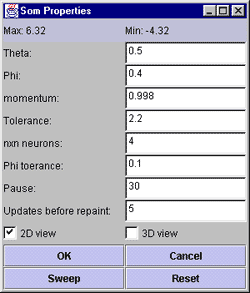
There are several different versions of the Kohonen Self-Organizing Map, but the principle is the same for all of them. Two different layers are described as the data-layer and the neuron-layer. The data-layer is the input in which we want to find some pattern or relations, and the neuron-layer is a collection of neurons with relations to other neurons in the layer as well as the data in the data-layer. The idea behind Self-Organizing Maps is that the neuron-layer through iteration steps called learning will make adaptations to the data-layer in a way that reduces the complexity and makes it easier for humans to analyse. The logical form of the neuron layer is often defined as a two-dimensional grid. Each neuron has a x co-ordinate and a y co-ordinate relative to the other neurons in the net. This grid, called lattice, is usually a quadratic or a hexagonal net. The algorithm presented in this application is a straight forward kohonen self-organizing map with a quadratic lattice and gauss neightbourhood function. It starts by initializing a mesh with the number of neurons set in the properties dialog. Since the algorithm implemented here are so straight forward, further details on the algorithm and properties of the Kohonen Self-organizing maps are left out from this help file. SOM Properties Theta is the size of the neighbourhood function. That is the size of the circumference around the best maching unit that will include other neurons to be moved in the direction of the inputvector. Too small values of theta will result in only individual neuron movements and thus the neuron-layer will not be arranged in a net structure. Since the net structure is one of the most important properties of Self-organizing maps, to small thetavalues is a waste of time. To high values will move all neurons towards the same point, resulting in a small heap of neurons that is moved in each iteration. Phi is the ammount a neuron within the neighborhood circumference will be moved towards the input-vector. Too small values of Phi will result in a neuron ordering much like the initial one, which is random and thus without any new information. Too large values will scatter the neurons all over the input area, leaving the result as random as it was at initialization. Values much higher than 1.0 makes no sence as the neurons will be moved beyond the input vector. Momentum is the ammount to reduce the learning parameters theta and phi after each iteration. Both will be their previous value times momentum. Too high momentum values will result in little global ordering of the map and more refining and too low values will do the oposit. Tolerance is the circumference around each neuron that will define the set of input-vectors that belongs to each neuron. Too high values will result in neurons with the same input vectors, and too low values will result in empty neurons. Tolerance is used when the sweep-button is clicked. It can be updated at any time. nxn neurons is the number of neurons in the lattice. Too few neurons in a large dataset results in a great loss of patterns (if any) because the few neurons can only cover a small area of the input area. To large values will slow the computation speed drastically without revealing any new information. Phi tolerance is a limit for how long the algorithm will keep running. When the phi limit has been reached, the algorithm terminates and the phi limit will have to be decremented in order to continue running. Too low values will keep the algorithm running when the learning parameters are so low that no changes are made. To high values will terminate the algorithm before the neurons has been ordered or the map has been refined, resulting in a loss of valuable information. Pause in the number of milliseconds to wait at each iteration. Too high values will slow the algorithm dramatically. Too low walues should not be a problem, but when the datasets are large, it seems that too low values (<10) will result in the algorithm going wild, and thus clicking a button will not fire an event at once. The pause field gives us an oportunity to view the ordering, growing and refinement of a map without everything going so fast that the algorithm has terminated before we know it :). Updates before repaint is a way to control how many iterations the algorithm will perform before updating the plot. The computation time for generating and painting a plot is oftem much larger than a simple iteration, so it might be wise to keep this number high in large datasets or large number of neurons. Finding the right values for all these properties can be a difficult task, and as a set of properties are found, they might not do so well on a different dataset. The default values seems to work all right for most datasets, but the number of neurons, pause and updates before repaint should be updated for larger datasets. It is very important to try out different properties for each dataset. All the values in the property window can be updated at runtime, except for the number of neurons and the views, which will be locked once the OK-Button is clicked.   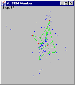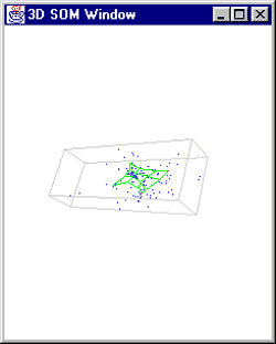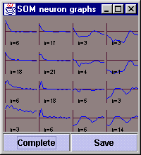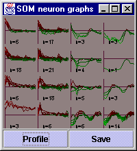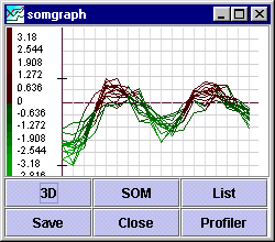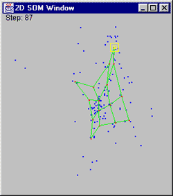SOM Functionality When the desired properties are inserted into the SOM properties window, a click on the OK-button will initialize the neuron layer with random values and generate the selected views. The plots are generated by a Principal components algorithm. The caption of the OK-button should now be changed to run and a click on this one will start the algorithm. The movement of the neurons can be viewed in the plots. It should be possible to press the stop-button at any time, resulting a freeze in the properties window and the plots. At this point, all properties can be changed except the number of neurons and the views. Click run to start the algorithm again. When stopped, it is possible to click the sweep-button. This will result in a window called "SOM neuron graphs" (see images to the right). This graph window will contain all the vectors belonging to a neuron after a sweep operation has been done (The circumference of this operation is set in the SOM properties window) expressed by eighter a mean graph or the complete set. The number in each component is the number of vectors belonging to this neuron. Clicking one of these graphs will pop up a somgraph (again pictured on the right), AND the neuron representing this SOM graph in the plots will be colored yellow (both 2D and 3D views). The somgraph has a SOM-button that can be used to apply further refinements to the dataset in this neuron. One of the most important properties of th self-organizing map is the way that its neurons are ordered. If the properties of the map is well chosen, neurons that are close neightbours in the node-grid will contain data that is closer related than nodes further away. By looking at the mean graphs of the data in the SOM neuron window, we can often se that neighbour neurons has a slightly similar curve.