Exercise 2 SC200 Spring 04.
Physical Problem : The Rayleigh-Benard Instability
The Model
Numerical Methods
Report
The Rayleigh-Benard Instability
We want to study the stability of a fluid situated between two plane and horizontal
plates maintained at two different temperatures, se Fig 1. Each plate is maintained
at an uniform temperature. We will try to evaluate the conditions and the nature of
the convective movement of the fluid.
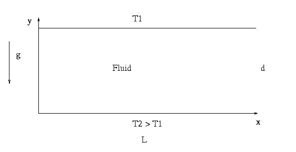
Fig 1.
In the case that the upper plate has a temperature higher then the temperature of the
lower plate, the thermal stratification is stable.
If we consider the opposite situation, where the upper plate is colder then the lower
plate, we have heavy fluid above lighter fluid and the fluid is only conditionally
stable. If the buoyance force due to Archimedes dominates the drag force due to
viscosity, the fluid will be unstable. If the drag force dominates, the fluid
will be stable. Thus, if the fluid is inviscid, it will be unstable
if T2 > T1 no matter how small the temperature difference is.
When the temperature gradient is over a critical value, rolls of convection
will appear between the two plates, a phenomenon which is called the Rayleigh-Benard
instability. Thus, as we increase the Rayleigh number defined by
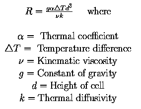
there is a transition from heat transfer through conduction to
heat transfer through convection. This is a buoyance driven convection and is
called thermal convection or Rayleigh-Benard convection. The critical Rayleigh number
for which this transition occurs can be estimated from the Nusselt number, defined
by
Nu= heat transfer/heat transfer by conduction.
We have that Nu=1 for R < Rc and then increases for R > Rc.
The Model
Boussinesq approximation
We will use Boussinesq approximation on our study of the R-B instability.
This means essentially that the density is assumed to be a function only of
the temperature and only in the buoyance term, while other fluid parameters such as
viscosity and thermal diffusivity are regarded as constants.
Such systems are governed by the Boussinesq equations
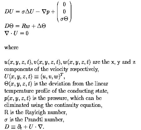
It is known that sufficiently close to the onset of convection and in a sufficiently
wide cell, the fluid motion is weakly three-dimensional in that only slow spatial
and temporal modulations of locally two-dimensional roll pattern can occour. The five
three-dimensional Boussinesq equations can then be replaced by a single two-dimensional
equation that describes the evolution of a complex amplitude or envelope function
whose phase and magnitude slowly modulate the sinusoidal oscillations of the rolls.
2D equation for the 3D
convection
A lowest-order nontrivial amplitude equation is obtained by multiple-scale
analysis of Boussinesq equations near onset. The perturbation is made in terms of
the small parameter

where Rc is the critical Rayleigh number at the Rayleigh-Benard instability
for a laterally infinite container. By including the rapid oscillations in a real
amplitude field  , where
 =
=  -1t is the
slow time variable, a rotationally invariant model equation can be derived.
This gives us the following model problem
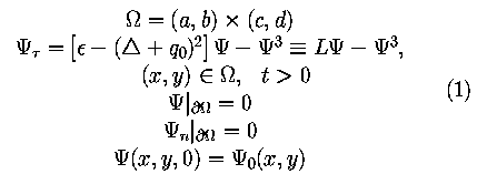
The model equation can be variationally derived from a Liapunov
functional

which decreases monotonically for all initial conditions. F is an
"energy" measure for solutions and provides a means of ordering possible roll
patterns according to their stability. The hydrodynamic variables can be
recovered from the two-dimensional field  as follows

where u0, w0 and  are the lowest eigenvalues of the
linearized Boussinesq system. Also the heat transport is known since the
Nusselt number can be computed from
  to within
O(
 ).
).
Numerical Methods
When solving the model (1) numerically, the Biharmonic BVP given in (2)
will have to be solved on every timestep.
This first part of Exercise 2
will therefore be finding numerical codes
for solving this boundary value problem and compare these codes.
First we will use a 2.nd order Finite Difference (FD) Scheme and then
a Spectral Galerkin Method. Then these two codes will be compared.

Finite Difference
Scheme
In netlib there is a code called
Bihar for solving (2) in rectangular domains. Download this code.
Choose one particular solution, and formulate a problem (2) which
has this solution.
Make a main program in
Fortran77/Fortran90. An alternative language may be used, provided that you are confident that
you will be able to correctly call the available Fortran subprograms.
This program should:
Give values to all parameters.
Set up the boundary conditions.
Call the subroutine bihar.
Call a subroutine which approximates the solution at an
arbitrary point (x,y).
Call a subroutine which calculates the L2 error and/or
max error.
This will involve making a subroutine to calculate these errors.
Write output data to a file.
Solve your problem from 2. numerically and plot your results.
Spectral
Legendre/Chebyshev Galerkin Method
A spectral Legendre/Chebyshev Galerkin method Bispec for
solving (2) in quadratic domains can be downloaded
here.
Go through questions 3. - 4. given above.
For simplicity you can take a = c = -1, b = d = 1 and study the
homogeneous problem (1) only (f2 = f3= 0).
Comparison of Finite Difference and Spectral
Method
Let Nx and Ny be the number of degrees of
freedom in the x- and y-
direction, respectively. What is the total number of degrees of freedom,
Ndof ? What is the computational cost of solving (2) with the
two methods expressed by Nx and Ny ?
Choose exact solution
u(x,y) = (sin(10 x))2(sin(10
 y))2
y))2
to problem (2). Let Nx = Ny, a = c = -1, b = d = 1. Plot the
L2 error vs. Ndof using logarithmic scale along
the ordinat.
Let
u(x,y) = (sin(c x))2(sin(c
 y))2
y))2
be an exact solution to problem (2).
Choose Nx = Ny = 200, a = c = -1, b = d = 1.
Let c = 1, 5, 10, 15, 20, . . ., 100.
Plot the L2 error vs. c using logarithmic scale along
the ordinat.
Based on your result in 3., how many degrees of freedom do
you need to resolve a "roll" with
10% accuracy
1% accuracy
0.1% accuracy
0.01% accuracy
when using the two methods ?
Compare the CPU time needed to resolve the "roll" patterns corresponding
to exact solutions
u(x,y) = (sin(10 x))2(sin(10
 y))2
y))2
u(x,y) = (sin(30 x))2(sin(30
 y))2
y))2
to (1) with 1% accuracy and 0.01% accuracy. Which method, 2.nd order
finite difference or spectral, would
you prefer to use ?
Time Dependent Equation
Having discretized the partial differential equation (PDE) in (1) spatially,
gives an initial value problem of ordinary differential equations (ODE)
with dimension Ndof to be solved. The linear 4.th order term
is very stiff and should be integrated implicitly.
Integrate the linear 4.th order term implicitly using implicit Euler and
nonlinear term explicitly using explicit Euler. This gives you a problem of
the form (2) to be solved at every timestep. Write down this problem.
Make two programs, one based the FD code bihar and one based on
the spectral code bispec, which solves the IBVP (1).
Vary  from 0.01 to 0.25. Plott
 vs.
vs.  averaged over the domain.
This should be done after the system has reached the steady state situation.
For which
  occurs the transition from conduction to convection. Use
L=8
 , d=4
, d=4 ,
,
 .
.
Let  = 0.25, L=8
 , d=4
, d=4 and
and
 .
.
Compute the evolution of the solution pattern of
 from
from  = 0 to
  = 800. Calculate
 averaged over the domain
for each time step. For
  = 0, 50, 100, 150, 200, 250, 300, 400, 500,
600, 700, 800 write the solution to a file and calculate
 . Plot
the solution pattern for some of these
  values. Comment your result.
Having calculated
  in 4. at every timestep, plot
 vs.
vs.  . Comment your results.
Make an animation showing the evolution of the solution pattern of
  .
.
Report
The report should be published on the web, it should be
complete and self contained and enable an interested reader to
repeat what you have done as well as carry on with possible
extensions of your investigation. The report must include :
- Summary
- Some background information related to the project, search the WEB
- A description of the project that you will undertake
- A description of the numerical methods used
and with complete answers to the given questions.
Difficulties and troubles that you encounter shall be described
to the extent that it will help the reader avoid similar problems.
This point also must include a discussion of your findings.
- Use graphics, curves and animations to illustrate your results.
- Conclusion
- References
Last updated: 10.02.04, petter.


 , where
 =
=  -1t is the
slow time variable, a rotationally invariant model equation can be derived.
This gives us the following model problem


 as follows

 are the lowest eigenvalues of the
linearized Boussinesq system. Also the heat transport is known since the
Nusselt number can be computed from
  to within
O(
 ).
).

 x))2(sin(10
 y))2
y))2  x))2(sin(c
 y))2
y))2  x))2(sin(10
 y))2
y))2  x))2(sin(30
 y))2
y))2  from 0.01 to 0.25. Plott
 vs.
vs.  averaged over the domain.
This should be done after the system has reached the steady state situation.
For which
  occurs the transition from conduction to convection. Use
L=8
 , d=4
, d=4 ,
,  .
. = 0.25, L=8
 , d=4
, d=4 and
and  .
.  from
from  = 0 to
  = 800. Calculate
 averaged over the domain
for each time step. For
  = 0, 50, 100, 150, 200, 250, 300, 400, 500,
600, 700, 800 write the solution to a file and calculate
 . Plot
the solution pattern for some of these
  values. Comment your result.
Having calculated
  in 4. at every timestep, plot
 vs.
vs.  . Comment your results.
Make an animation showing the evolution of the solution pattern of
  .
.