|
Application - 2 Coulomb Crystals
Background
The purpose of this resaerch is to investigate the structure and
dynamics of so-called ions trapped in a electric and magnetic field
(Paul
Trap). Ion Coulomb Crystals are the solid state of plasma containing only
particles of the same sign of charge. One-component plasma (OCP's)
consist only of one single ion species. OCP's at
low temperatures have been studied intensively theoretically and
during the last 10 years also experimentally with laser cooled ions in
traps. Ions in free space repel each other
due to Coulomb force repulsion and expand to infinity. In a trap
(Fig. below) an
additional attractive potential keeps the system bounded. For certain
parameters of the potential the most favorable energetic configuration
(the state with lowest energy) of
the ions will be to organize them self in a linear string.
Such a string is at present one of the most promising candidates for
implementing a quantum processor, which have the potential of solving
classical exponential problems in linear time.
In classical mechanics the dynamics of the particles is determined by Newtons 2. law,

The forces can be calculated from the potential energy function

The potential is a sum of electrostatic repulsions and trap attractions,

where  is the coordinate of
particle i. The mass Mi is defined in [amu],
qi, qj are defined in [e]
and is the coordinate of
particle i. The mass Mi is defined in [amu],
qi, qj are defined in [e]
and  . .
From experimentalists we learn that a typical trap parameter:

For example, assuming a weaker  one
can observe a transition from a 1-dimensional string (41 Ca+, MPEG, 322KB) to a 2-dimesional
zig-zag line (42 Ca+, MPEG, 320KB)
by increasing the number of ions. one
can observe a transition from a 1-dimensional string (41 Ca+, MPEG, 322KB) to a 2-dimesional
zig-zag line (42 Ca+, MPEG, 320KB)
by increasing the number of ions.
We investigate for increasing numbers of ions
whether they converge to shell structure or not,
especially for bi-crystals. Our computer simulation are performed
with the object-oriented component based molecular
dynamics framework ProtoMol. In order to
solve larger-sized simulation problems
we use the multi-grid method, which performs for large
system about 100-600 times faster and a maximum relative force error of
order 10-3 compared to the direct method. For the
convergence to shell or lattice structure this
accuracy is appropriated. If needed, one may run some few final steps
with a more accurate method. This ongoing project is a collaboration
with Michael Drewsen who provides
experimental data.
ProtoMol
ProtoMol is an object-oriented component based framework for molecular
dynamics simulations. The framework supports the CHARMM 19 and 28a2 force
fields and is able to process PDB, PSF, XYZ and DCD trajectory files. It
is designed for high flexibility, easy extendibility and maintenance, and
high performance demands, including parallelization. The technique of
multiple time-stepping has been used to improve long-term efficiency, and
the use of fast electrostatic force evaluation algorithms like plain Ewald,
Particle Mesh Ewald, and Multigrid summation further improves
performance. Longer time steps are possible using MOLLY, Langevin Molly
and Hybrid Monte Carlo, Nose-Hoover, and Langevin integrators. In
addition, ProtoMol has been designed to interact with VMD, a visualization
engine developed by the University of Illinois that is used for displaying
large biomolecular systems in three dimensions. ProtoMol is free
distributed software, and the source code will be included.
ProtoMol is been developed in collaboration with J.A. Izaguirre and members of
the LCLS Group; CSE
Department, University of Notre Dame,
Indiana, USA.
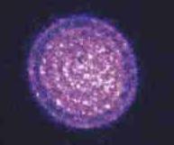
Computer Simulation and Results
Newtons 2. law is solved by a Leap-Frog integrator scheme with Nose-Hoover
thermostat, starting with an initial temperature of ~1mK and cooled
down to ~1uK. The simulation runs represent 1ms with an integration
step of 100ns. The start configuration has a different density
distribution compared to the final configuration, such that the
temperature will temporally increase in the beginning of the
simulation. The Coulombic part was computed directly for
small system sizes, whereas a multi-grid
method was used for the largest
system size.


|


|
|
2057 Ca+40;
Direct method
(config,
434K archive)
|


|


 a
b
a
b
|
| 1029 Ca+40 and 1028 A2+80;
Direct method
(config,
454K archive)
|


|


|
| 20288 Ca+40;
Multigrid, FE=4.10-3
(config,
1.4M archive)
|


|


|
| 17752 Ca+40 and 2536 A2+80;
Multigrid, FE=4.10-3
(config,
1.4M archive)
|


|


|
| 15216 Ca+40 and 5072 A2+80;
Multigrid, FE=4.10-3
(config,
1.4M archive)
|


|


 a
b
a
b
|
| 10144 Ca+40 and 10144 A2+80;
Multigrid, FE=4.10-3
(config,
1.4M archive)
|


|


|
| 5072 Ca+40 and 15216 A2+80;
Multigrid, FE=4.10-3
(config,
1.4M archive)
|


|


|
| 2536 Ca+40 and 17752 A2+80;
Multigrid, FE=4.10-3
(config,
1.4M archive)
|


|


|
| 20288 A2+80;
Multigrid, FE=4.10-3
(config,
1.4M archive)
|


|


 m (1ms),
m (10ns)
m (1ms),
m (10ns)

|
| 100000 Ca+40;
Multigrid, FE=4.10-3
(config,
6.5M archive)
|


|


 m (1ms),
m (10ns)
m (1ms),
m (10ns)

|
| 50000 Ca+40 and 50000 A2+80;
Multigrid, FE=4.10-3
(config,
6.5M archive)
|


|


 m (1ms)
m (10ns)
m (1ms)
m (10ns)

|
| 100000 A2+80;
Multigrid, FE=4.10-3
(config,
6.5M archive)
|
Related Links
TTP5 Presentation - Status Report
- Bergen 25/6 2001 (PDF)
- Tromsø 14/12 2001 (PDF)
- Oslo 11/06 2002 (PDF)
- Fevik 30/08 2002 (PDF)
Last modified: .
|
